
# Imports
import pandas as pd
import numpy as np
#make sure to install sklearn in your terminal first!
from sklearn.model_selection import train_test_split
from sklearn.preprocessing import MinMaxScaler, StandardScaler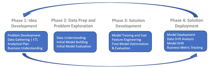
The above data science lifecycle is a simple overview of the steps involved in most data science projects. Its important to note that the steps are not always linear, and you may need to iterate through them multiple times. The focus of this chapter is on the data preparation step, which is crucial for building a successful machine learning model. Subsequent chapters will cover the other steps in more detail.
Phase I
Working to develop a model than can predict cereal quality rating...
-What is the target variable?
-Assuming we are able to optimize and make recommendations how does this translate into a business context?
-Prediction problem: Classification or Regression?
-Independent Business Metric: Assuming that higher ratings results in higher sales, can we predict which new cereals that enter the market over the next year will perform the best?
Phase II
Data Preparation
Variable Classes (Numeric versus Categorical)
Ensuring that variables are of the correct type before working with machine learning models is essential for several reasons. Machine learning algorithms expect input data to be in specific formats, such as numerical values for regression models or categorical values for classification models. Incorrect variable types can lead to errors during model training and evaluation, as well as inaccurate predictions. For instance, attempting to perform mathematical operations on string data types will result in runtime errors. Additionally, proper variable types facilitate appropriate preprocessing steps, such as encoding categorical variables or scaling numerical features. By verifying and correcting variable types beforehand, we can avoid potential issues, ensure the integrity of the data, and improve the overall performance and reliability of the machine learning models. We also need to check to make sure categorical levels are balanced, if not we may need to be modified.
#read in the cereal dataset, you should have this locally or you can use the URL linking to the class repo below
cereal = pd.read_csv("https://raw.githubusercontent.com/UVADS/DS-3001/main/data/cereal.csv")

cereal.info() # Let's check the structure of the dataset and see if we have any issues with variable classes
#usually it's converting things to category
---------------------------------------------------------------------------
NameError                                 Traceback (most recent call last)
Cell In[1], line 2
      1 #read in the cereal dataset, you should have this locally or you can use the URL linking to the class repo below
----> 2 cereal = pd.read_csv("https://raw.githubusercontent.com/UVADS/DS-3001/main/data/cereal.csv")
      4 cereal.info() # Let's check the structure of the dataset and see if we have any issues with variable classes
      5 #usually it's converting things to category

NameError: name 'pd' is not defined
#Looks like columns 1,2,11 and 12 need to be converted to category
Column_index_list = [1,2,11,12]
cereal.iloc[:,Column_index_list]= cereal.iloc[:,Column_index_list].astype('category')
#iloc accesses the index of a dataframe, bypassing having to manually type in the names of each column
cereal.dtypes #another way of checking the structure of the dataset. Simpler, but does not give an index/tmp/ipykernel_5493/3417620518.py:4: FutureWarning: Setting an item of incompatible dtype is deprecated and will raise in a future error of pandas. Value '0 25
1 0
2 25
3 25
4 25
..
72 25
73 25
74 25
75 25
76 25
Name: vitamins, Length: 77, dtype: category
Categories (3, int64): [0, 25, 100]' has dtype incompatible with int64, please explicitly cast to a compatible dtype first.
cereal.iloc[:,Column_index_list]= cereal.iloc[:,Column_index_list].astype('category')
/tmp/ipykernel_5493/3417620518.py:4: FutureWarning: Setting an item of incompatible dtype is deprecated and will raise in a future error of pandas. Value '0 3
1 3
2 3
3 3
4 3
..
72 3
73 2
74 1
75 1
76 1
Name: shelf, Length: 77, dtype: category
Categories (3, int64): [1, 2, 3]' has dtype incompatible with int64, please explicitly cast to a compatible dtype first.
cereal.iloc[:,Column_index_list]= cereal.iloc[:,Column_index_list].astype('category')
#Let's take a closer look at mfr
cereal.mfr.value_counts() #value_counts() simply displays variable counts as a vertical table.#Usually don't want more than 5 groups, so we should collapse this factor
#Keep the large groups (G, K) and group all the smaller categories as "Other"
top = ['K','G']
cereal.mfr = (cereal.mfr.apply(lambda x: x if x in top else "Other")).astype('category')
#lambda is a small anonymous function that can take any number of arguments but can only have one expression
#a simple lambda function is lambda a: a+10, if we passed 5 to this we would get back 15
#lambda functions are best used inside of another function, like in this example when it is used inside the apply function
#to use an if function in a lambda statement, the True return value comes first (x), then the if statement, then else, and then the False return
cereal.mfr.value_counts() #This is a lot bettercereal.type.value_counts() #looks goodcereal.vitamins.value_counts() #also goodcereal.weight.value_counts() #what about this one? ... Not a categorical variable groupings so it does not matter right nowScale/Center
Scaling and normalizing variables are crucial steps in preparing data for machine learning models because they ensure that all features contribute equally to the model’s performance. Without scaling, features with larger ranges can dominate the learning process, leading to biased models. Normalization, on the other hand, transforms the data to a common scale, typically between 0 and 1, which helps in speeding up the convergence of gradient descent algorithms. Both techniques improve the numerical stability of the model and enhance the performance of algorithms that rely on distance metrics, such as k-nearest neighbors and support vector machines. Overall, scaling and normalizing variables lead to more accurate and efficient machine learning models.
#Centering and Standardizing Data
sodium_sc = StandardScaler().fit_transform(cereal[['sodium']])
#reshapes series into an appropriate argument for the function fit_transform: an array

sodium_sc[:10] #essentially taking the zscores of the data, here are the first 10 values
array([[-0.35630563],
[-1.73708742],
[ 1.20457813],
[-0.23623765],
[ 0.48417024],
[ 0.24403427],
[-0.41633962],
[ 0.60423822],
[ 0.48417024],
[ 0.60423822]])Normalizing the numeric values
#Let's look at min-max scaling, placing the numbers between 0 and 1.
sodium_n = MinMaxScaler().fit_transform(cereal[['sodium']])
sodium_n[:10]
array([[0.40625 ],
[0.046875],
[0.8125 ],
[0.4375 ],
[0.625 ],
[0.5625 ],
[0.390625],
[0.65625 ],
[0.625 ],
[0.65625 ]])#Let's check just to be sure the relationships are the same
cereal.sodium.plot.density()<Axes: ylabel='Density'>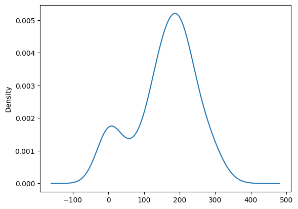
pd.DataFrame(sodium_n).plot.density() #Checks out!<Axes: ylabel='Density'>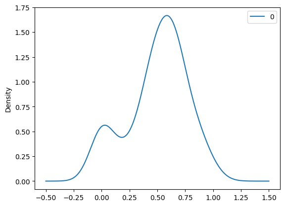
#Now we can move forward in normalizing the numeric values and create a index based on numeric columns:
abc = list(cereal.select_dtypes('number'))
#select function to find the numeric variables and create a list

cereal[abc] = MinMaxScaler().fit_transform(cereal[abc])
cereal #notice the difference in the range of values for the numeric variablesOne-hot Encoding
One-hot encoding is a technique used to convert categorical variables into a numerical format that machine learning models can understand and process. Categorical variables often contain non-numeric data, such as labels or categories, which cannot be directly used by most machine learning algorithms. One-hot encoding addresses this by creating binary columns for each category, where each column represents a unique category and contains a 1 if the category is present and a 0 otherwise. This transformation allows the model to interpret categorical data without assuming any ordinal relationship between the categories, which could otherwise introduce bias. By using one-hot encoding, we ensure that the categorical information is accurately represented, improving the model’s ability to learn from the data and make accurate predictions
# Next let's one-hot encode those categorical variables

category_list = list(cereal.select_dtypes('category')) #select function to find the categorical variables and create a list

cereal_1h = pd.get_dummies(cereal, columns = category_list)
#get_dummies encodes categorical variables into binary by adding in indicator column for each group of a category
#and assigning it 0 if false or 1 if true
cereal_1h #see the difference? This is one-hot encoding!Baseline/Prevalence
Prevalence in machine learning models refers to the proportion of instances in a dataset that belong to a particular class, typically the positive class in binary classification problems. It is a measure of how common or frequent a specific outcome or class is within the dataset. Prevalence is important because it provides insight into the class distribution, which can significantly impact model performance and evaluation. For example, in imbalanced datasets where one class is much more prevalent than the other, standard performance metrics like accuracy can be misleading. Understanding prevalence helps in selecting appropriate evaluation metrics, such as precision, recall, or the F1 score, and in applying techniques like resampling or class weighting to address class imbalance and improve model performance.
#This is essentially the target to which we are trying to out perform with our model. Percentage is represented by the positive class.
#Rating is continuous, but we are going to turn it into a Boolean to be used for classification by selecting the top quartile of values.

cereal_1h.boxplot(column= 'rating', vert= False, grid=False)
cereal_1h.rating.describe() #notice the upper quartile of values will be above 0.43 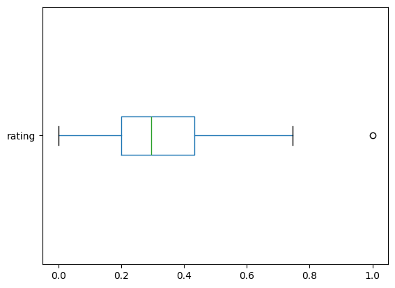
#add this as a predictor instead of replacing the numeric version
cereal_1h['rating_f'] = pd.cut(cereal_1h.rating, bins = [-1,0.43,1], labels =[0,1])
#If we want two segments we input three numbers, start, cut and stop values

cereal_1h #notice the new column rating_f, it is now binary based on if the continuous value is above 0.43 or not#So now let's check the prevalence
prevalence = cereal_1h.rating_f.value_counts()[1]/len(cereal_1h.rating_f)
#value_count()[1] pulls the count of '1' values in the column (values above .43)
prevalence #gives percent of values above .43 which is equivalent to the prevalence or our baselinenp.float64(0.2727272727272727)#let's just double check this
print(cereal_1h.rating_f.value_counts())
print(21/(21+56)) #looks good!rating_f
0 56
1 21
Name: count, dtype: int64
0.2727272727272727
Dropping Variables and Partitioning
Partitioning datasets in preparation for machine learning is essential to evaluate and validate the performance of models effectively. By dividing the data into distinct subsets, typically training, validation, and test sets, we can ensure that the model is trained, tuned, and tested on different portions of the data. The training set is used to fit the model, allowing it to learn patterns and relationships within the data. The validation set is used to fine-tune model parameters and select the best model configuration, helping to prevent overfitting by providing an unbiased evaluation during the training process. Finally, the test set is used to assess the model’s performance on unseen data, providing an estimate of how well the model will generalize to new, real-world data. This partitioning helps in building robust, reliable models and ensures that the evaluation metrics reflect the model’s true performance.
#Divide up our data into three parts, Training, Tuning, and Test but first we need to...
#clean up our dataset a bit by dropping the original rating variable and the cereal name since we can't really use them

cereal_dt = cereal_1h.drop(['name','rating'],axis=1) #creating a new dataframe so we don't delete these columns from our working environment.
cereal_dt# Now we partition
Train, Test = train_test_split(cereal_dt, train_size = 55, stratify = cereal_dt.rating_f)
#stratify perserves class proportions when splitting, reducing sampling error print(Train.shape)
print(Test.shape)(55, 21)
(22, 21)
#Now we need to use the function again to create the tuning set
Tune, Test = train_test_split(Test,  train_size = .5, stratify= Test.rating_f)
#check the prevalance in all groups, they should be all equivalent in order to eventually build an accurate model
print(Train.rating_f.value_counts())
print(15/(40+15))rating_f
0 40
1 15
Name: count, dtype: int64
0.2727272727272727
print(Tune.rating_f.value_counts())
print(3/(8+3)) #good
rating_f
0 8
1 3
Name: count, dtype: int64
0.2727272727272727
print(Test.rating_f.value_counts())
print(3/(8+3)) #same as above, good job!
rating_f
0 8
1 3
Name: count, dtype: int64
0.2727272727272727
from sklearn.tree import DecisionTreeClassifier
from sklearn.metrics import precision_score

# Initialize the DecisionTreeClassifier
dtree = DecisionTreeClassifier()

# Fit the model on the training data
dtree.fit(X_train, y_train)

# Predict on the test data
y_pred_dtree = dtree.predict(X_test)

# Calculate precision
precision = precision_score(y_test, y_pred_dtree)

print(f'Precision: {precision}')
---------------------------------------------------------------------------
NameError Traceback (most recent call last)
Cell In[26], line 8
5 dtree = DecisionTreeClassifier()
7 # Fit the model on the training data
----> 8 dtree.fit(X_train, y_train)
10 # Predict on the test data
11 y_pred_dtree = dtree.predict(X_test)
NameError: name 'X_train' is not definedNow you try!
job = pd.read_csv("https://raw.githubusercontent.com/DG1606/CMS-R-2020/master/Placement_Data_Full_Class.csv")
job.head()
from io import StringIO
import requests
url="https://query.data.world/s/ttvvwduzk3hwuahxgxe54jgfyjaiul"
s=requests.get(url).text
c=pd.read_csv(StringIO(s))
c.head()