kNN Evaluation Example

#Imports
import pandas as pd
import numpy as np
import matplotlib.pyplot as plt
#When importing libraries that have several packages with corresponding functions
#If you know you will only need to use one specific function from a certain package
#It is better to simply import it directly, as seen below, since it is more efficient and allows for greater simplicity later on
from sklearn.model_selection import train_test_split 
from sklearn.preprocessing import StandardScaler
from sklearn.neighbors import KNeighborsClassifier
from sklearn import metrics

#Read in the data from the github repo, you should also have this saved locally...
bank_data = pd.read_csv("https://raw.githubusercontent.com/UVADS/DS-3001/main/07_ML_Eval_Metrics/bank.csv")

#Let's take a look
print(bank_data.dtypes)
bank_data.head()

#Drop any rows that are incomplete (rows that have NA's in them)
bank_data = bank_data.dropna() #dropna drops any rows with any NA value by default

#In this example our target variable is the column 'signed up', lets convert it to a category so we can work with it
bank_data['signed up'] = bank_data['signed up'].astype("category")

bank_data.dtypes #looks good

#Before we form our model, we need to prep the data...
#First let's scale the features we will be using for classification
#Remember this essentially just converts the raw values to z-scores, standardizing them
bank_data[["age","duration","balance"]]= StandardScaler().fit_transform(bank_data[["age","duration","balance"]])

#Next we are going to partition the data, but first we need to isolate the independent and dependent variables
X = bank_data[["age","duration","balance"]]  #independent variables
y = bank_data['signed up']                  #dependent variable
#Sometimes you will see only the values be taken using the function .values however this is simply personal preference 
#Since there are several independent variables, I decided to keep the labels in order to distinguish a specific independent variable if needed.

#Now we partition, using our good old friend train_test_split 
#The train_size parameter can be passed a percent or an exact number depending on the circumstance and desired output
#In this case an exact number does not necessarily matter so let's split by percent 
X_train, X_test, y_train, y_test = train_test_split(X, y, train_size=0.70, stratify = y, random_state=21)
#Remember specifying the parameter 'stratify' is essential to perserve class proportions when splitting, reducing sampling error 
#Also set the random_state so our results can be reproducible 

#Now we need to use the function again to create the tuning set
#We want equally sized sets here so let's pass 50% to train_size
X_tune, X_test, y_tune, y_test = train_test_split(X_test,y_test,  train_size = 0.50, stratify = y_test,random_state=49)
#In this example, we are just going to use the train and tune data.

#Finally, it's time to build our model!
#Here is a function we imported at the beginning of the script,
#In this case it allows us to create a knn model and specify number of neighbors to 10
bank_3NN = KNeighborsClassifier(n_neighbors=10)
#Now let's fit our knn model to the training data
bank_3NN.fit(X_train, y_train)
#note this is simply a model, let's apply it to something and get results!

#This is how well our model does when applied to the tune set
bank_3NN.score(X_tune, y_tune) #This is the probability that our model predicted the correct output based on given inputs, not bad...

#In order to take a look at other metrics, we first need to extract certain information from our model
#Let's retrieve the probabilities calculated from our tune set
bank_prob1 = bank_3NN.predict_proba(X_tune) #This function gives percent probability for both class (0,1)
bank_prob1[:5] #both are important depending on our question, in this example we want the positive class

#Now let's retrieve the predictions, based on the tuning set...
bank_pred1 = bank_3NN.predict(X_tune)
bank_pred1[:5] #looks good, notice how the probabilities above correlate with the predictions below

#Building a dataframe for simplicity, including everything we extracted and the target
final_model= pd.DataFrame({'neg_prob':bank_prob1[:, 0], 'pred':bank_pred1,'target':y_tune, 'pos_prob':bank_prob1[:, 1]})
#Now everything is in one place!

final_model.head() #Nice work!

#Now let's create a confusion matrix by inputing the predications from our model and the original target
metrics.confusion_matrix(final_model.target,final_model.pred) #looks good, but simplistic...

#Let's make it a little more visually appealing so we know what we are looking at 
#This function allows us to include labels which will help us determine number of true positives, fp, tn, and fn
metrics.ConfusionMatrixDisplay.from_predictions(final_model.target,final_model.pred, display_labels = [False, True], colorbar=False)
#Ignore the color, as there is so much variance in this example it really is not telling us anything

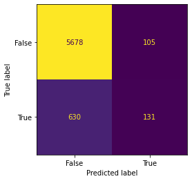
#What if we want to adjust the threshold to produce a new set of evaluation metrics
#Let's build a function so we can make the threshold whatever we want, not just the default 50%
def adjust_thres(x,y,z):
  #x=pred_probablities, y=threshold, z=test_outcome
  thres = (np.where(x > y, 1,0))
  #np.where is essentially a condensed if else statement. The first argument is the condition, then the true output, then the false output
  return metrics.ConfusionMatrixDisplay.from_predictions(z,thres, display_labels = [False, True], colorbar=False)

# Give it a try with a threshold of .35
adjust_thres(final_model.pos_prob,.35,final_model.target)
#What's the difference? Try different percents now, what happens?

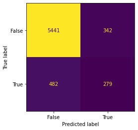
#Now let's use our model to obtain an ROC Curve and the AUC
metrics.RocCurveDisplay.from_predictions(final_model.target, final_model.pos_prob)
#Set labels and midline...
plt.plot([0, 1], [0, 1],'r--')
plt.ylabel('True Positive Rate')
plt.xlabel('False Positive Rate')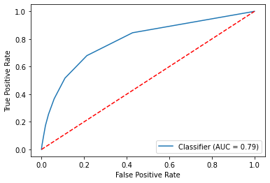

#Let's extract the specific AUC value now
metrics.roc_auc_score(final_model.target, final_model.pos_prob) #Looks good!

#Determine the log loss
metrics.log_loss(final_model.target, final_model.pos_prob)

#Get the F1 Score
metrics.f1_score(final_model.target, final_model.pred)

#Extra metrics
print(metrics.classification_report(final_model.target, final_model.pred)) #Nice Work!