#Imports
import pandas as pd
import numpy as np
import matplotlib.pyplot as plt
import graphviz

from sklearn.model_selection import train_test_split,GridSearchCV,RepeatedStratifiedKFold
from sklearn import metrics
from sklearn.metrics import ConfusionMatrixDisplay
from sklearn.preprocessing import OrdinalEncoder
from sklearn.tree import DecisionTreeClassifier, export_graphviz
CART Example using Sklearn: Use a new Dataset, complete preprocessing, use three data
partitions: Training, Tuning and Testing, and build a model!
#Read in the data from the github repo, you should also have this saved locally...
winequality = pd.read_csv("https://raw.githubusercontent.com/UVADS/DS-3001/main/data/winequality-red-ddl.csv")
#Let's take a look...
print(winequality.info())
print(winequality.head())<class 'pandas.core.frame.DataFrame'>
RangeIndex: 1599 entries, 0 to 1598
Data columns (total 13 columns):
# Column Non-Null Count Dtype
--- ------ -------------- -----
0 fixed acidity 1599 non-null float64
1 volatile acidity 1575 non-null float64
2 citric acid 1595 non-null float64
3 residual sugar 1586 non-null float64
4 chlorides 1587 non-null float64
5 free sulfur dioxide 1583 non-null float64
6 total sulfur dioxide 1574 non-null float64
7 density 1579 non-null float64
8 pH 1597 non-null float64
9 sulphates 1591 non-null float64
10 alcohol 1589 non-null float64
11 quality 1581 non-null float64
12 text_rank 1581 non-null object
dtypes: float64(12), object(1)
memory usage: 162.5+ KB
None
fixed acidity volatile acidity citric acid residual sugar chlorides \
0 11.6 0.580 0.66 2.20 0.074
1 10.4 0.610 0.49 2.10 0.200
2 7.4 1.185 0.00 4.25 0.097
3 10.4 0.440 0.42 1.50 0.145
4 8.3 1.020 0.02 3.40 0.084
free sulfur dioxide total sulfur dioxide density pH sulphates \
0 10.0 47.0 1.00080 3.25 0.57
1 5.0 16.0 0.99940 3.16 0.63
2 5.0 14.0 0.99660 3.63 0.54
3 34.0 48.0 0.99832 3.38 0.86
4 6.0 11.0 0.99892 3.48 0.49
alcohol quality text_rank
0 9.0 3.0 poor
1 8.4 3.0 poor
2 10.7 3.0 poor
3 9.9 3.0 poor
4 11.0 3.0 poor
#This will be our target variable
print(winequality.text_rank.value_counts())
text_rank
ave 678
average-ish 630
good 193
poor-ish 53
excellent 17
poor 10
Name: count, dtype: int64
Preprocessing
#drop quality column since it predicts text_rank perfectly
winequality= winequality.drop(columns='quality')
Missing Data
#Let's see if we have any NA's
print(winequality.isna().sum()) #show location of NA's by variable
fixed acidity 0
volatile acidity 24
citric acid 4
residual sugar 13
chlorides 12
free sulfur dioxide 16
total sulfur dioxide 25
density 20
pH 2
sulphates 8
alcohol 10
text_rank 18
dtype: int64
#Let's just drop them
winequality= winequality.dropna()
print(winequality.info()) #Lost some rows, but should be fine with this size dataset<class 'pandas.core.frame.DataFrame'>
Index: 1482 entries, 0 to 1580
Data columns (total 12 columns):
# Column Non-Null Count Dtype
--- ------ -------------- -----
0 fixed acidity 1482 non-null float64
1 volatile acidity 1482 non-null float64
2 citric acid 1482 non-null float64
3 residual sugar 1482 non-null float64
4 chlorides 1482 non-null float64
5 free sulfur dioxide 1482 non-null float64
6 total sulfur dioxide 1482 non-null float64
7 density 1482 non-null float64
8 pH 1482 non-null float64
9 sulphates 1482 non-null float64
10 alcohol 1482 non-null float64
11 text_rank 1482 non-null object
dtypes: float64(11), object(1)
memory usage: 150.5+ KB
None
Collapsing the target
#Let's collapse text_rank now into only two classes
winequality.text_rank.value_counts() #What should we combine?
text_rank
ave 635
average-ish 583
good 186
poor-ish 51
excellent 17
poor 10
Name: count, dtype: int64#Condense everything into either average or excellent
winequality["text_rank"]= winequality["text_rank"].replace(['good','average-ish','poor-ish','poor'], ['excellent','ave','ave','ave'])
print(winequality["text_rank"].value_counts()) #Great!text_rank
ave 1279
excellent 203
Name: count, dtype: int64
#check the prevalence
print(203/(1279+203))
0.1369770580296896
#Before we move forward, we have one more preprocessing step
#We must encode text_rank to become a integer array variable as that is the only type sklearn decision trees can currently take
winequality[["text_rank"]] = OrdinalEncoder().fit_transform(winequality[["text_rank"]])
print(winequality["text_rank"].value_counts()) #nice
text_rank
0.0 1279
1.0 203
Name: count, dtype: int64
Splitting the Data
#split independent and dependent variables
X= winequality.drop(columns='text_rank')
y= winequality.text_rank
#There is not a easy way to create 3 partitions using the train_test_split
#so we are going to use it twice. Mostly because we want to stratify on the variable we are working to predict. What does that mean?
#what should I stratify by??? Our Target!
X_train, X_test, y_train, y_test = train_test_split(X, y, train_size=0.70, stratify= y, random_state=21)
X_tune, X_test, y_tune, y_test = train_test_split(X_test,y_test, train_size = 0.50,stratify= y_test, random_state=49)
Let’s Build the Model
#Three steps in building a ML model
#Step 1: Cross validation process- the process by which the training data will be used to build the initial model must be set. As seen below:

kf = RepeatedStratifiedKFold(n_splits=10,n_repeats =5, random_state=42)
# number - number of folds
# repeats - number of times the CV is repeated, takes the average of these repeat rounds

# This essentially will split our training data into k groups. For each unique group it will hold out one as a test set
# and take the remaining groups as a training set. Then, it fits a model on the training set and evaluates it on the test set.
# Retains the evaluation score and discards the model, then summarizes the skill of the model using the sample of model evaluation scores we choose
#What score do we want our model to be built on? Let's use:
#AUC for the ROC curve - remember this is measures how well our model distiguishes between classes
#Recall - this is sensitivity of our model, also known as the true positive rate (predicted pos when actually pos)
#Balanced accuracy - this is the (sensitivity + specificity)/2, or we can just say it is the number of correctly predicted data points
print(metrics.SCORERS.keys()) #find themdict_keys(['explained_variance', 'r2', 'max_error', 'neg_median_absolute_error', 'neg_mean_absolute_error', 'neg_mean_absolute_percentage_error', 'neg_mean_squared_error', 'neg_mean_squared_log_error', 'neg_root_mean_squared_error', 'neg_mean_poisson_deviance', 'neg_mean_gamma_deviance', 'accuracy', 'top_k_accuracy', 'roc_auc', 'roc_auc_ovr', 'roc_auc_ovo', 'roc_auc_ovr_weighted', 'roc_auc_ovo_weighted', 'balanced_accuracy', 'average_precision', 'neg_log_loss', 'neg_brier_score', 'adjusted_rand_score', 'rand_score', 'homogeneity_score', 'completeness_score', 'v_measure_score', 'mutual_info_score', 'adjusted_mutual_info_score', 'normalized_mutual_info_score', 'fowlkes_mallows_score', 'precision', 'precision_macro', 'precision_micro', 'precision_samples', 'precision_weighted', 'recall', 'recall_macro', 'recall_micro', 'recall_samples', 'recall_weighted', 'f1', 'f1_macro', 'f1_micro', 'f1_samples', 'f1_weighted', 'jaccard', 'jaccard_macro', 'jaccard_micro', 'jaccard_samples', 'jaccard_weighted'])
#Define score, these are the keys we located above. This is what the models will be scored by
scoring = ['roc_auc','recall','balanced_accuracy']
#Step 2: Usually involves setting a hyper-parameter search. This is optional and the hyper-parameters vary by model.
#define parameters, we can use any number of the ones below but let's start with only max depth
#this will help us find a good balance between under fitting and over fitting in our model
param={"max_depth" : [1,2,3,4,5,6,7,8,9,10,11],
#"splitter":["best","random"],
#"min_samples_split":[5,10,15,20,25],
#"min_samples_leaf":[5,10,15,20,25],
#"min_weight_fraction_leaf":[0,0.1,0.2,0.3,0.4,0.5,0.6,0.7,0.8,0.9],
#"max_features":["auto","log2","sqrt",None],
#"max_leaf_nodes":[10,20,30,40,50],
#'min_impurity_decrease':[0.00005,0.0001,0.0002,0.0005,0.001,0.0015,0.002,0.005,0.01],
#'ccp_alpha' :[.001, .01, .1]
}#Step 3: Train the Model
#Classifier model we will use
cl= DecisionTreeClassifier(random_state=1000)
#Set up search for best decisiontreeclassifier estimator across all of our folds based on roc_auc
search = GridSearchCV(cl, param, scoring=scoring, n_jobs=-1, cv=kf,refit='roc_auc')
#execute search on our training data, this may take a few seconds ...
model = search.fit(X_train, y_train)Let’s see how we did
#Retrieve the best estimator out of all parameters passed, based on highest roc_auc
best = model.best_estimator_
print(best) #depth of 5, good
DecisionTreeClassifier(max_depth=5, random_state=1000)
#Plotting the decision tree for the best estimator
dot_data = export_graphviz(best, out_file =None,
               feature_names =X.columns, #feature names from dataset
               filled=True,
                rounded=True,
                class_names = ['ave','excellent']) #classification labels

graph=graphviz.Source(dot_data)
graph
Loading...
#What about the specific scores (roc_auc, recall, balanced_accuracy)? Let's try and extract them to see what we are working with ...
print(model.cv_results_) #This is a dictionary and in order to extract info we need the keys
Fetching long content....
#Which one of these do we need?
print(model.cv_results_.keys()) #get mean_test and std_test for all of our scores, and will need our param_max_depth as well
dict_keys(['mean_fit_time', 'std_fit_time', 'mean_score_time', 'std_score_time', 'param_max_depth', 'params', 'split0_test_roc_auc', 'split1_test_roc_auc', 'split2_test_roc_auc', 'split3_test_roc_auc', 'split4_test_roc_auc', 'split5_test_roc_auc', 'split6_test_roc_auc', 'split7_test_roc_auc', 'split8_test_roc_auc', 'split9_test_roc_auc', 'split10_test_roc_auc', 'split11_test_roc_auc', 'split12_test_roc_auc', 'split13_test_roc_auc', 'split14_test_roc_auc', 'split15_test_roc_auc', 'split16_test_roc_auc', 'split17_test_roc_auc', 'split18_test_roc_auc', 'split19_test_roc_auc', 'split20_test_roc_auc', 'split21_test_roc_auc', 'split22_test_roc_auc', 'split23_test_roc_auc', 'split24_test_roc_auc', 'split25_test_roc_auc', 'split26_test_roc_auc', 'split27_test_roc_auc', 'split28_test_roc_auc', 'split29_test_roc_auc', 'split30_test_roc_auc', 'split31_test_roc_auc', 'split32_test_roc_auc', 'split33_test_roc_auc', 'split34_test_roc_auc', 'split35_test_roc_auc', 'split36_test_roc_auc', 'split37_test_roc_auc', 'split38_test_roc_auc', 'split39_test_roc_auc', 'split40_test_roc_auc', 'split41_test_roc_auc', 'split42_test_roc_auc', 'split43_test_roc_auc', 'split44_test_roc_auc', 'split45_test_roc_auc', 'split46_test_roc_auc', 'split47_test_roc_auc', 'split48_test_roc_auc', 'split49_test_roc_auc', 'mean_test_roc_auc', 'std_test_roc_auc', 'rank_test_roc_auc', 'split0_test_recall', 'split1_test_recall', 'split2_test_recall', 'split3_test_recall', 'split4_test_recall', 'split5_test_recall', 'split6_test_recall', 'split7_test_recall', 'split8_test_recall', 'split9_test_recall', 'split10_test_recall', 'split11_test_recall', 'split12_test_recall', 'split13_test_recall', 'split14_test_recall', 'split15_test_recall', 'split16_test_recall', 'split17_test_recall', 'split18_test_recall', 'split19_test_recall', 'split20_test_recall', 'split21_test_recall', 'split22_test_recall', 'split23_test_recall', 'split24_test_recall', 'split25_test_recall', 'split26_test_recall', 'split27_test_recall', 'split28_test_recall', 'split29_test_recall', 'split30_test_recall', 'split31_test_recall', 'split32_test_recall', 'split33_test_recall', 'split34_test_recall', 'split35_test_recall', 'split36_test_recall', 'split37_test_recall', 'split38_test_recall', 'split39_test_recall', 'split40_test_recall', 'split41_test_recall', 'split42_test_recall', 'split43_test_recall', 'split44_test_recall', 'split45_test_recall', 'split46_test_recall', 'split47_test_recall', 'split48_test_recall', 'split49_test_recall', 'mean_test_recall', 'std_test_recall', 'rank_test_recall', 'split0_test_balanced_accuracy', 'split1_test_balanced_accuracy', 'split2_test_balanced_accuracy', 'split3_test_balanced_accuracy', 'split4_test_balanced_accuracy', 'split5_test_balanced_accuracy', 'split6_test_balanced_accuracy', 'split7_test_balanced_accuracy', 'split8_test_balanced_accuracy', 'split9_test_balanced_accuracy', 'split10_test_balanced_accuracy', 'split11_test_balanced_accuracy', 'split12_test_balanced_accuracy', 'split13_test_balanced_accuracy', 'split14_test_balanced_accuracy', 'split15_test_balanced_accuracy', 'split16_test_balanced_accuracy', 'split17_test_balanced_accuracy', 'split18_test_balanced_accuracy', 'split19_test_balanced_accuracy', 'split20_test_balanced_accuracy', 'split21_test_balanced_accuracy', 'split22_test_balanced_accuracy', 'split23_test_balanced_accuracy', 'split24_test_balanced_accuracy', 'split25_test_balanced_accuracy', 'split26_test_balanced_accuracy', 'split27_test_balanced_accuracy', 'split28_test_balanced_accuracy', 'split29_test_balanced_accuracy', 'split30_test_balanced_accuracy', 'split31_test_balanced_accuracy', 'split32_test_balanced_accuracy', 'split33_test_balanced_accuracy', 'split34_test_balanced_accuracy', 'split35_test_balanced_accuracy', 'split36_test_balanced_accuracy', 'split37_test_balanced_accuracy', 'split38_test_balanced_accuracy', 'split39_test_balanced_accuracy', 'split40_test_balanced_accuracy', 'split41_test_balanced_accuracy', 'split42_test_balanced_accuracy', 'split43_test_balanced_accuracy', 'split44_test_balanced_accuracy', 'split45_test_balanced_accuracy', 'split46_test_balanced_accuracy', 'split47_test_balanced_accuracy', 'split48_test_balanced_accuracy', 'split49_test_balanced_accuracy', 'mean_test_balanced_accuracy', 'std_test_balanced_accuracy', 'rank_test_balanced_accuracy'])
#Let's extract these scores, using our function!

#Scores:

auc = model.cv_results_['mean_test_roc_auc']
recall= model.cv_results_['mean_test_recall']
bal_acc= model.cv_results_['mean_test_balanced_accuracy']

SDauc = model.cv_results_['std_test_roc_auc']
SDrecall= model.cv_results_['std_test_recall']
SDbal_acc= model.cv_results_['std_test_balanced_accuracy']

#Parameter:
depth= np.unique(model.cv_results_['param_max_depth']).data

#Build DataFrame:
final_model = pd.DataFrame(list(zip(depth, auc, recall, bal_acc,SDauc,SDrecall,SDbal_acc)),
               columns =['depth','auc','recall','bal_acc','aucSD','recallSD','bal_accSD'])

#Let's take a look
final_model.style.hide(axis='index')
Loading...
#Warning!
#If we used multiple params... you won't be able to get the scores as easily
#Say we wanted to get the scores based on max_depth still, but this time we used the parameter ccp_alpha as well
#Use the np.where function to search for the indices where the other parameter equals their best result, in this say it is .001
#This is an example code to find auc: #model.cv_results_['mean_test_roc_auc'][np.where((model.cv_results_['param_ccp_alpha'] == .001))]
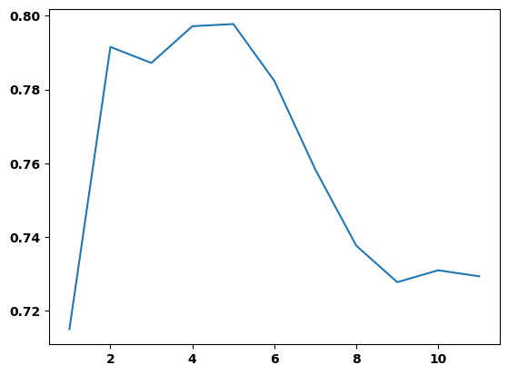
#Essentially takes indices and resulting scores where the best parameters were used #Check the depth ...
print(plt.plot(final_model.depth,final_model.auc)) #5 does in fact have the highest (best) AUC![<matplotlib.lines.Line2D object at 0x000001A23875E550>]
Variable Importance
#Variable importance for the best estimator, how much weight does each feature have in determining the classification?
varimp=pd.DataFrame(best.feature_importances_,index = X.columns,columns=['importance']).sort_values('importance', ascending=False)
print(varimp)
importance
alcohol 0.387980
sulphates 0.125469
pH 0.102023
volatile acidity 0.095476
density 0.076325
fixed acidity 0.068555
citric acid 0.034814
chlorides 0.033507
total sulfur dioxide 0.030891
free sulfur dioxide 0.023970
residual sugar 0.020989
#Graph variable importance
plt.figure(figsize=(10,7))
print(varimp.importance.nlargest(7).plot(kind='barh')) #Alcohol has the largest impact by far!
Let’s use the model to predict and the evaluate the performance
#Confusion Matrix time! Passing our tuning data into our best model, let's see how we do ...
print(ConfusionMatrixDisplay.from_estimator(best,X_tune,y_tune, display_labels = ['ave','excellent'], colorbar=False))
Let’s play with the threshold, what do we see
## Adjust threshold function
def adjust_thres(model,X,y_true, thres):
  #model= best estimator, X= feature vairables, y_true= target variables, thres = threshold
  y_pred = (model.predict_proba(X)[:,1] >= thres).astype(np.int32) #essentially changes the prediction cut off to our desired threshold
  return metrics.ConfusionMatrixDisplay.from_predictions(y_true,y_pred, display_labels = ['ave','excellent'], colorbar=False)
#Where should we change the threshold to see a difference...
print(pd.DataFrame(model.predict_proba(X_tune)[:,1]).plot.density())#Let's try .1 as our new threshold ...
print(adjust_thres(best,X_tune, y_tune,.1))Accuracy Score
print(best.score(X_test,y_test)) #Pretty precise, nice!---------------------------------------------------------------------------
NameError Traceback (most recent call last)
/Users/bpugs/Desktop/DS-3001/08_DT_Class/Decision Trees.ipynb Cell 45' in <cell line: 1>()
----> <a href='vscode-notebook-cell:/Users/bpugs/Desktop/DS-3001/08_DT_Class/Decision%20Trees.ipynb#ch0000179?line=0'>1</a> print(best.score(X_test,y_test))
NameError: name 'best' is not definedprint(best.score(X_tune,y_tune)) #same with tuning setFeature Engineering:
#What feature should we look at?
print(winequality.describe())
fixed acidity volatile acidity citric acid residual sugar \
count 1482.000000 1482.000000 1482.000000 1482.000000
mean 8.320243 0.528870 0.269744 2.548853
std 1.718001 0.180651 0.194912 1.431911
min 4.600000 0.120000 0.000000 0.900000
25% 7.100000 0.390000 0.090000 1.900000
50% 7.900000 0.520000 0.260000 2.200000
75% 9.200000 0.640000 0.420000 2.600000
max 15.900000 1.580000 1.000000 15.500000
chlorides free sulfur dioxide total sulfur dioxide density \
count 1482.000000 1482.000000 1482.000000 1482.000000
mean 0.087808 16.018893 46.965587 0.996764
std 0.048015 10.419929 33.141959 0.001868
min 0.012000 1.000000 6.000000 0.990070
25% 0.070000 7.000000 22.000000 0.995653
50% 0.080000 14.000000 38.000000 0.996800
75% 0.091000 22.000000 63.000000 0.997857
max 0.611000 72.000000 289.000000 1.003690
pH sulphates alcohol
count 1482.000000 1482.000000 1482.000000
mean 3.311505 0.659777 10.406545
std 0.153826 0.168406 1.064761
min 2.740000 0.330000 8.400000
25% 3.210000 0.550000 9.500000
50% 3.310000 0.620000 10.100000
75% 3.400000 0.730000 11.100000
max 4.010000 2.000000 14.900000
# How about total sulfur dioxide ...
print(plt.hist(winequality['total sulfur dioxide'], width=15, bins = 15))
#Get the five number summary, and some...
print(winequality['total sulfur dioxide'].describe())#make a new dataframe so we can preserve our working environment
winequality1 = winequality.copy(deep=True)#lump total sulfure dioxide to below and above its median (38)
winequality1['total sulfur dioxide']=pd.cut(winequality1['total sulfur dioxide'],(0,37,300), labels = ("low","high"))#transform it to a numeric variable so we can use it in sklearn decision tree
winequality1[["total sulfur dioxide"]] = OrdinalEncoder().fit_transform(winequality1[["total sulfur dioxide"]])#Separate features and target
X1=winequality1.drop(columns='text_rank')
y1=winequality1.text_rank#Data splitting
X_train1, X_test1, y_train1, y_test1 = train_test_split(X1, y1, train_size=0.70, stratify= y1, random_state=21)
X_tune1, X_test1, y_tune1, y_test1 = train_test_split(X_test1,y_test1, train_size = 0.50,stratify= y_test1, random_state=49)#define search, model, paramameters and scoring will be the same...
search_eng = GridSearchCV(cl, param, scoring=scoring, n_jobs=-1, cv=kf,refit='roc_auc')
#execute search
model_eng = search_eng.fit(X_train1, y_train1)#Take a look at our best estimator for depth this time
best_eng = model_eng.best_estimator_
print(best_eng) #4, a different depth!#Check out the mean and standard deviation test scores again ...
auc = model_eng.cv_results_['mean_test_roc_auc']
recall= model_eng.cv_results_['mean_test_recall']
bal_acc= model_eng.cv_results_['mean_test_balanced_accuracy']
SDauc = model_eng.cv_results_['std_test_roc_auc']
SDrecall= model_eng.cv_results_['std_test_recall']
SDbal_acc= model_eng.cv_results_['std_test_balanced_accuracy']
#Parameter:
depth= np.unique(model_eng.cv_results_['param_max_depth']).data
#Build DataFrame:
final_model = pd.DataFrame(list(zip(depth, auc, recall, bal_acc,SDauc,SDrecall,SDbal_acc)),
columns =['depth','auc','recall','bal_acc','aucSD','recallSD','bal_accSD'])
#Let's take a look
final_model.style.hide(axis='index')Compare the confusion matrices from the two models
#First model
print(ConfusionMatrixDisplay.from_estimator(best,X_tune,y_tune,colorbar=False))
#New engineered model
print(ConfusionMatrixDisplay.from_estimator(best_eng,X_tune1,y_tune1,colorbar=False)) #Better tpr and tnr!We can also review the variable importance
#First model
print(pd.DataFrame(best.feature_importances_,index = X.columns,columns=['importance']).sort_values('importance', ascending=False))
#Engineered model
print(pd.DataFrame(best_eng.feature_importances_,index = X1.columns,columns=['importance']).sort_values('importance', ascending=False))
#Smaller model so less variables are considered in the decision making for better or worse...
Predict with test, how did we do?
#Original model
print(ConfusionMatrixDisplay.from_estimator(best,X_test,y_test,colorbar=False))
#New engineered model
print(ConfusionMatrixDisplay.from_estimator(best_eng,X_test1,y_test1,colorbar=False)) #Ultimately, very similar resultsHow about accuracy score?
#Original model
print(best.score(X_test,y_test)) #accuracy
#Engineered model
print(best_eng.score(X_test1,y_test1)) #Basically the sameAnother example with a binary dataset this time!
#Load in new dataset
pregnancy = pd.read_csv("https://raw.githubusercontent.com/UVADS/DS-3001/main/data/pregnancy.csv")
#Let's get familiar with the data
print(pregnancy.info())
print(pregnancy.head())<class 'pandas.core.frame.DataFrame'>
RangeIndex: 2000 entries, 0 to 1999
Data columns (total 16 columns):
# Column Non-Null Count Dtype
--- ------ -------------- -----
0 Pregnancy Test 2000 non-null int64
1 Birth Control 2000 non-null int64
2 Feminine Hygiene 2000 non-null int64
3 Folic Acid 2000 non-null int64
4 Prenatal Vitamins 2000 non-null int64
5 Prenatal Yoga 2000 non-null int64
6 Body Pillow 2000 non-null int64
7 Ginger Ale 2000 non-null int64
8 Sea Bands 2000 non-null int64
9 Stopped buying ciggies 2000 non-null int64
10 Cigarettes 2000 non-null int64
11 Smoking Cessation 2000 non-null int64
12 Stopped buying wine 2000 non-null int64
13 Wine 2000 non-null int64
14 Maternity Clothes 2000 non-null int64
15 PREGNANT 2000 non-null int64
dtypes: int64(16)
memory usage: 250.1 KB
None
Pregnancy Test Birth Control Feminine Hygiene Folic Acid \
0 1 0 0 0
1 1 0 0 0
2 1 0 0 0
3 0 0 0 0
4 0 0 0 0
Prenatal Vitamins Prenatal Yoga Body Pillow Ginger Ale Sea Bands \
0 1 0 0 0 0
1 1 0 0 0 0
2 0 0 0 0 1
3 0 0 0 1 0
4 0 1 0 0 0
Stopped buying ciggies Cigarettes Smoking Cessation Stopped buying wine \
0 0 0 0 0
1 0 0 0 0
2 0 0 0 0
3 0 0 0 0
4 0 0 0 1
Wine Maternity Clothes PREGNANT
0 0 0 1
1 0 0 1
2 0 0 1
3 0 0 1
4 0 0 1
#We want to build a classifier that can predict whether a shopper is pregnant
#based on the items they buy so we can direct-market to that customer if possible.

print(pregnancy.PREGNANT.sum())
print(len(pregnancy.PREGNANT))

print((1- pregnancy.PREGNANT.sum()/len(pregnancy.PREGNANT)))
#What does .72 represent in this context? Prevalence of not being pregnant
560
2000
0.72
reformat for exploration purposes
#Creating a vertical dataframe for the pregnant variable, just stacking the variables on top of each other.
#First get the column names of features then use pd.melt based on the Pregnancy variable
feature_cols = pregnancy.drop(columns='PREGNANT').columns
pregnancy_long = df = pd.melt(pregnancy, id_vars='PREGNANT', value_vars=feature_cols,
             var_name='variable', value_name='value')


print(pregnancy_long.head())
PREGNANT variable value
0 1 Pregnancy Test 1
1 1 Pregnancy Test 1
2 1 Pregnancy Test 1
3 1 Pregnancy Test 0
4 1 Pregnancy Test 0
See what the base rate likihood of pregnancy looks like for each variable
# Calculate the probability of being pregnant by predictor variable.
# First let's create a new list to store our probability data
data=[]
#loop through features and retrieve probability of pregnancy for whether it is bought or not bought
#Since the data is binary you can take the average to get the probability.
for col in feature_cols:
    x = pregnancy.groupby([col])['PREGNANT'].mean()
    data.extend([[col,0,x[0]],[col,1,x[1]]])
base_rate = pd.DataFrame(data, columns = ['Var', 'Value','prob_pregnant'])
base_rate['prob_not_pregnant']= 1-base_rate.prob_pregnant
print(base_rate)
Var Value prob_pregnant prob_not_pregnant
0 Pregnancy Test 0 0.254441 0.745559
1 Pregnancy Test 1 0.848837 0.151163
2 Birth Control 0 0.327859 0.672141
3 Birth Control 1 0.058989 0.941011
4 Feminine Hygiene 0 0.321212 0.678788
5 Feminine Hygiene 1 0.085714 0.914286
6 Folic Acid 0 0.234792 0.765208
7 Folic Acid 1 0.952381 0.047619
8 Prenatal Vitamins 0 0.236741 0.763259
9 Prenatal Vitamins 1 0.742690 0.257310
10 Prenatal Yoga 0 0.273647 0.726353
11 Prenatal Yoga 1 0.826087 0.173913
12 Body Pillow 0 0.276596 0.723404
13 Body Pillow 1 0.538462 0.461538
14 Ginger Ale 0 0.261717 0.738283
15 Ginger Ale 1 0.623762 0.376238
16 Sea Bands 0 0.271845 0.728155
17 Sea Bands 1 0.651163 0.348837
18 Stopped buying ciggies 0 0.255113 0.744887
19 Stopped buying ciggies 1 0.605634 0.394366
20 Cigarettes 0 0.305413 0.694587
21 Cigarettes 1 0.097959 0.902041
22 Smoking Cessation 0 0.261523 0.738477
23 Smoking Cessation 1 0.797101 0.202899
24 Stopped buying wine 0 0.242458 0.757542
25 Stopped buying wine 1 0.600000 0.400000
26 Wine 0 0.317612 0.682388
27 Wine 1 0.086154 0.913846
28 Maternity Clothes 0 0.239956 0.760044
29 Maternity Clothes 1 0.677596 0.322404
Build the model
#Split between features and target and do a three way split
X_preg=pregnancy.drop(columns='PREGNANT')
y_preg=pregnancy.PREGNANT
X_train_preg, X_test_preg, y_train_preg, y_test_preg = train_test_split(X_preg, y_preg, train_size=0.70, stratify= y_preg, random_state=21)
X_tune_preg, X_test_preg, y_tune_preg, y_test_preg = train_test_split(X_test_preg,y_test_preg,  train_size = 0.50,stratify= y_test_preg, random_state=49)
#This time we are going to use a different technique to complete our hyper-parameter search
#define our model, still using the same classifier as before
cl2=DecisionTreeClassifier(random_state=1000)
#prune our model using minimal cost-complexity pruning, this is an algorithm used to prune a tree to avoid over-fitting
path = cl2.cost_complexity_pruning_path(X_train_preg, y_train_preg)
ccp_alphas, impurities = path.ccp_alphas, path.impurities#Let's do some exploration into what cost complexity alpha gives the best results without overfitting or underfitting ...
fig, ax = plt.subplots()
#In the following plot, the maximum effective alpha value is removed, because it is the trivial tree with only one node
fig.set_size_inches(18.5, 10.5, forward=True)
plt.xticks(ticks=np.arange(0.00,0.06,.0025))
ax.plot(ccp_alphas[:-1], impurities[:-1], marker="o", drawstyle="steps-post")
ax.set_xlabel("effective alpha")
ax.set_ylabel("total impurity of leaves")
ax.set_title("Total Impurity vs effective alpha for training set")
#As alpha increases, more of the tree is pruned, which increases the total impurity of its leaves.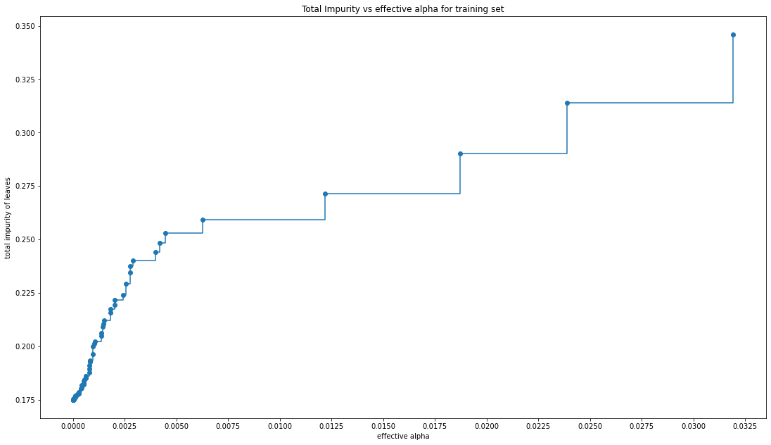
#run through all of our alphas and create fitted decision tree classifiers for them so we can explore even further
clfs = []
for ccp_alpha in ccp_alphas:
    clf = DecisionTreeClassifier(random_state=0, ccp_alpha=ccp_alpha)
    clf.fit(X_train_preg, y_train_preg)
    clfs.append(clf)
#we remove the last element in clfs and ccp_alphas, because it is the trivial tree with only one node.
clfs = clfs[:-1]
ccp_alphas = ccp_alphas[:-1]

# Here we show that the number of nodes and tree depth decreases as alpha increases, makes sense since the tree is getting smaller
node_counts = [clf.tree_.node_count for clf in clfs]
depth = [clf.tree_.max_depth for clf in clfs]
fig, ax = plt.subplots(2, 1)
ax[0].plot(ccp_alphas, node_counts, marker="o", drawstyle="steps-post")
ax[0].set_xlabel("alpha")
ax[0].set_ylabel("number of nodes")
ax[0].set_title("Number of nodes vs alpha")
ax[1].plot(ccp_alphas, depth, marker="o", drawstyle="steps-post")
ax[1].set_xlabel("alpha")
ax[1].set_ylabel("depth of tree")
ax[1].set_title("Depth vs alpha")
fig.set_size_inches(18.5, 10.5, forward=True)
plt.xticks(ticks=np.arange(0.00,0.06,.0025))
fig.tight_layout()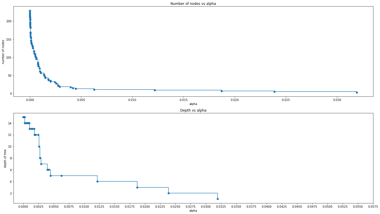
#When ccp_alpha is set to zero and keeping the other default parameters of DecisionTreeClassifier,
#the tree overfits, leading to a 100% training accuracy and less testing accuracy.
#As alpha increases, more of the tree is pruned, thus creating a decision tree that generalizes better.
#Let's try and find the alpha where we get the highest accuracy for both training and testing data simultaneously
train_scores = [clf.score(X_train_preg, y_train_preg) for clf in clfs]
test_scores = [clf.score(X_tune_preg, y_tune_preg) for clf in clfs]
fig, ax = plt.subplots()
ax.set_xlabel("alpha")
ax.set_ylabel("accuracy")
ax.set_title("Accuracy vs alpha for training and testing sets")
ax.plot(ccp_alphas, train_scores, marker="o", label="train", drawstyle="steps-post")
ax.plot(ccp_alphas, test_scores, marker="o", label="test", drawstyle="steps-post")
ax.legend()
plt.xticks(ticks=np.arange(0.00,0.06,.0025))
fig.set_size_inches(18.5, 10.5, forward=True)
plt.show()
#In this example, setting ccp_alpha=0.001 maximizes the testing accuracy.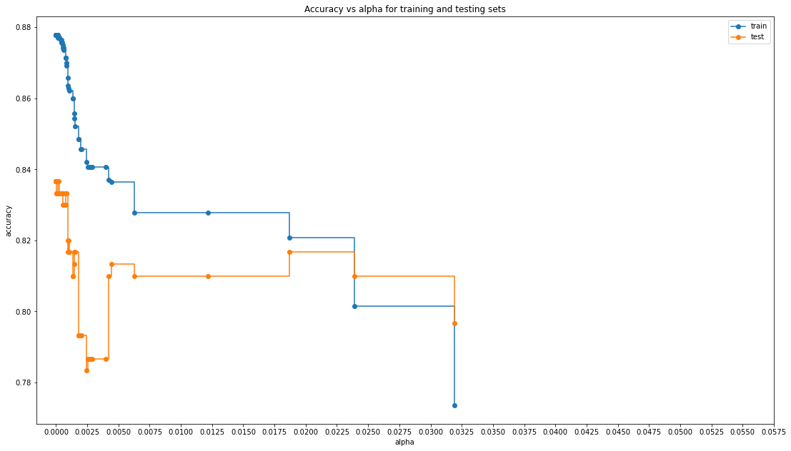
#Let's take a look to get an exact value
tree=DecisionTreeClassifier(ccp_alpha= 0.001)
tree.fit(X_train_preg,y_train_preg)0.8433333333333334Variable Importance
#Shows the reduction in error provided by including a given variable
print(pd.DataFrame(tree.feature_importances_,index = X_preg.columns,columns=['importance']).sort_values('importance', ascending=False))
importance
Folic Acid 0.282159
Prenatal Vitamins 0.157229
Pregnancy Test 0.117627
Maternity Clothes 0.097533
Stopped buying wine 0.073541
Feminine Hygiene 0.064128
Birth Control 0.063039
Smoking Cessation 0.030172
Ginger Ale 0.029064
Wine 0.024732
Cigarettes 0.023650
Stopped buying ciggies 0.018642
Sea Bands 0.013422
Body Pillow 0.005061
Prenatal Yoga 0.000000
Test the accuracy
tree.score(X_test_preg,y_test_preg) #84% accurate, nice!0.8433333333333334#Confusion matrix
ConfusionMatrixDisplay.from_estimator(tree,X_test_preg,y_test_preg, colorbar = False)<sklearn.metrics._plot.confusion_matrix.ConfusionMatrixDisplay at 0x7f99bba25ee0>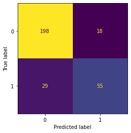
Hit Rate or True Classification Rate, Detection Rate and ROC
# The error rate is defined as a classification of "Pregnant" when
# this is not the case, and vice versa. It's the sum of all the
# values where a column contains the opposite value of the row.
pred_preg = tree.predict(X_test_preg)
tn, fp, fn, tp = metrics.confusion_matrix(y_test_preg,pred_preg).ravel()
# The error rate divides this figure by the total number of data points
# for which the forecast is created.
print("Hit Rate/True Error Rate = "+ str((fp+fn)/len(y_test_preg)*100))
Hit Rate/True Error Rate = 15.666666666666668
#Detection Rate is the rate at which the algo detects the positive class in proportion to the entire classification A/(A+B+C+D) where A is poss poss
print("Detection Rate = " +str((tp)/len(y_test_preg)*100)) #want this to be higher but there is only so high it can go...
Detection Rate = 18.333333333333332
#Building the evaluation ROC and AUC using the predicted and original target variables
metrics.RocCurveDisplay.from_predictions(y_test_preg,pred_preg)
#Set labels and midline...
plt.plot([0, 1], [0, 1],'r--')
plt.ylabel('True Positive Rate')
plt.xlabel('False Positive Rate')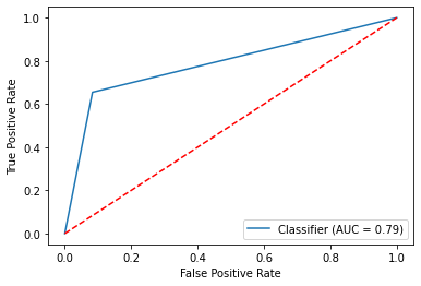
#We can adjust using a if else statement and the predicted prob, now we have to be 75% sure to classify as pregnant
pred_adjusted = (tree.predict_proba(X_test_preg)[:,1] >= .75).astype(np.int32)
metrics.RocCurveDisplay.from_predictions(y_test_preg,pred_adjusted)
plt.plot([0, 1], [0, 1],'r--')
plt.ylabel('True Positive Rate')
plt.xlabel('False Positive Rate')
We can also prune the tree to make it less complex
#Set parameters for our model, this time let's use the complexity parameter or the value of the splitting criterion
param2={"max_depth" : [1,2,3,4,5,6,7],
        #"splitter":["best","random"],
        #'criterion': ['gini','entropy'],
        #"min_samples_split":[5,10,15,20,25],
        #"min_samples_leaf":[2,4,6,8,10],
        #"min_weight_fraction_leaf":[0,0.1,0.2,0.3,0.4,0.5,0.6,0.7,0.8,0.9],
        #"max_features":["auto","log2","sqrt",None],
        #"max_leaf_nodes":[10,20,30,40,50],
        #'min_impurity_decrease':[0.00005,0.0001,0.0002,0.0005,0.001,0.0015,0.002,0.005,0.01],
        'ccp_alpha' : [.001]
           }
# set our model
cl2=DecisionTreeClassifier(random_state=1000)
# set scoring
scoring2= ['roc_auc','recall','balanced_accuracy']
# define search
search_preg = GridSearchCV(cl2, param2, scoring=scoring2, n_jobs=-1, cv=kf,refit='roc_auc')
#execute search
model_preg = search_preg.fit(X_train_preg, y_train_preg)

#Let's get our results!
best_preg= model_preg.best_estimator_
print(best_preg) #Now only has a max depth of 7
print(tree.tree_.max_depth) #A lot better than 14!#let's take a look
dot_data = export_graphviz(best_preg, out_file =None,
feature_names =X_preg.columns, #column names of our features
filled=True,
rounded=True,
class_names=['no','yes']) #classification labels
graph_preg=graphviz.Source(dot_data)
graph_pregbest_preg.score(X_test_preg,y_test_preg) #Same accuracy as well!---------------------------------------------------------------------------
NameError Traceback (most recent call last)
/Users/bpugs/Desktop/DS-3001/08_DT_Class/Decision Trees.ipynb Cell 101' in <cell line: 1>()
----> <a href='vscode-notebook-cell:/Users/bpugs/Desktop/DS-3001/08_DT_Class/Decision%20Trees.ipynb#ch0000149?line=0'>1</a> best_preg.score(X_test_preg,y_test_preg)
NameError: name 'best_preg' is not defined